Math Review

Despite the advanced tooling we have at our disposal, it is often helpful to understand the mathematics fundamentals behind the algorithms we use. These fundamentals become especially important when interpreting and evaluating our results.

Notation

There's a lot of math short hands and symbols that makes it easier to express and quantify ideas. Let's go over a few that you might encounter in Data Science literature.

Summation

The summation symbol is the capital Greek letter Sigma used for summing values in a series. The i represents the index and m, n represents the lower and upper bound respectively.

$$\sum_{i=m}^{n} y_i = y_m + ... + y_n$$

Factorials, Permutations and Combinations

The factorial of a positive integer \(n\) is denoted as \(n!\) and represents the product of all numbers equal to or less than n. For instance, 5 factorial is \(5! = 5 \times 4 \times 3 \times 2 \times 1\).

Factorials are important for counting permutations, the different ways a set can be arranged. To calculate the number of permutations, we need to know the total number of elements in the set and the number of elements taken at a time. One of the assumptions is that each element can only be used once in the ordering.

$$P(n, r) = \frac{n!}{(n - r)!}$$

where \(n\) is the total number of elements while \(r\) is the number of elements taken at a time.

Consider a competition between 10 people where one person will be selected as first place, another as second place and another as third place. In this case, \(n=10\) is the number of contestants. We are interested in the different combinations of first, second and third place, thus \(r=3\). The number of permutations is calculated as:

$$P(10, 3) = \frac{10!}{(10 - 3)!}$$

Combinations count the number of arrangements when order doesn't matter. If there was no distinction between first, second and third place, we can use the combinations formula to calculate the number of arrangements for top 3 out of our 10 contestants.

$${n \choose r} = \frac{n!}{(n - r) ! r!} = \frac{P(n, r)}{r!}$$

We can read the left hand side as n choose r.

Logarithms

The logarithm function (commonly abbreviated as log) is the inverse function to exponentiation. The logarithm of positive real number \(x\) with base \(b\) is the exponent that \(b\) needs to be raised to yield \(x\). This value is expressed as \(\log_b x\).

For instance, \(2^3 = 8\) informs us that \(\log_2 8 = 3\).

There are some very useful logarithm laws (also called logarithm identities) to help illustrate this relationship.

Euler's constant \(e\)

Euler's constant \(e\) is approxiamately 2.718. It is also used as the base for the natural logarithm. The natural logarithm of \(x\) is \(\log_e x\), which is also denoted as \(\ln x\).

\(e\) can actually be calculated as the sum of an infinite series:

$$ e = \sum_{i=0}^{\infty} \frac{1}{i!}$$

Statistics

The Wikipedia definition states that statistics is the discipline that concerns the collection, organization, analysis, interpretation and presentation of data. That actually sounds a lot like what a Data Scientist does! As such, it should come to no surprise that several fundamental Data Science principles, methodologies and even Machine Learning algorithms are heavily rooted in Statistics.

Probability Theory

Probability theory is the field of study in mathematics concerned with probability. Two very important concepts in probability theory are probability distributions and random variables.

Probability distributions are functions which map events to their occurrence probabilities. In statistics, events are any possible outcome. We call the set of all possible events/outcomes the sample space.

A random variable is a variable whose values are outcomes of a random phenomenon.

For example, we can model single, fair dice rolls as a random variable with the sample space \(\{1,2,3,4,5,6\}\). Rolling any number in the sample space is an event.

We usually use capital letters such as \(X\) to denote random variables. If we let lowercase \(x\) be an event, then \(P(x)\) is the probability of \(x\) occurring. We denote the sample space of all possible events as \(S\).

Probability Distributions

There are two types of probability distributions:

The difference between these two distributions is the composition of their sample space. The sample space of a discrete distribution is composed of discrete values, whereas the sample space of a continuous distribution is composed of continuous values within a range.

We typically express probability distributions using:

PDF/PMF are functions which maps the random variable taking on a single value to its occurrence probability. If the dice roll is our random variable, then we would characterize its Probability Mass Function as a function which maps the event of the dice landing on one number to its occurrence probability.

In this case, \(S = \{1,2,3,4,5,6\}\) and \(P(x) = \frac{1}{6}\) for all \(x\) in our sample space.

For a function to qualify as a probability density/mass function, the probability of any given event must be between 0 and 1 and the probability of all possible events must equal 1.

Cumulative Density Functions map event \(x\) to the probability of an event less than or equal to \(x\) occurring. For continuous distributions, the CDF is the integral of the PDF - the area under the curve. We can thus deduce the PDF from the CDF by taking its derivative. For discrete distributions, the CDF is the sum of all values equal or smaller than \(x\).

In the case of the dice roll, the CDF can be calculated as \(P(X \leq x) = \Sigma_{\forall i \in S, i \leq x} P(i)\).

Expectation, Variance and Co-Variance

Expectation: This is the average value we expect to get if the experiment was repeated many times. If we get 1 dollar for flipping a head in a fair coin and nothing for flipping a tails, then our expected earning is 0.5 dollars from a single coin flip. We represent the expected value of random variable \(X\) as \(E(X)\).

Variance: The variance is a measure of how far the observed values are spread apart. The variance of observations \(y_1, ... y_n\) can be calculated as \(\sum_{i=1}^{n} (y_i - \bar{y})^2\). The bar in \(\bar{y}\) represents the average observed value of \(y\). We represent the variance of random variable \(X\) as \(Var(X)\) which can be calculated using \(E(X^2) - E(X)^2\).

Co-variance: Co-variance measures the joint variability between two random variables. The covariance between random variables \(X, Y\) is calculated as \(Cov(X, Y) = E(XY) - E(X)E(Y)\).

Common Probability Distributions

Some probability distributions are so common that they have earned names for themselves. This list introduces only a few of them.

Poisson Distribution

The Poisson distribution is used to model count data, i.e. the number of times an event of interest occurs. We can use Poisson distribution to model the number of car accidents or the number of purchases for a certain item.

The particular parameter of interest in the Poisson distribution is the rate of events occurring (usually represented by \(\lambda\), pronounced lambda). Typically, this represents the average rate of event occurrence within a set time interval.

The Poisson model makes a few assumptions:

The PMF for Poisson distribution is \(P(X=x) = \frac{\lambda^x e^{-\lambda}}{x!}\). The mean and variance both equal to \(\lambda\).

Binomial Distribution

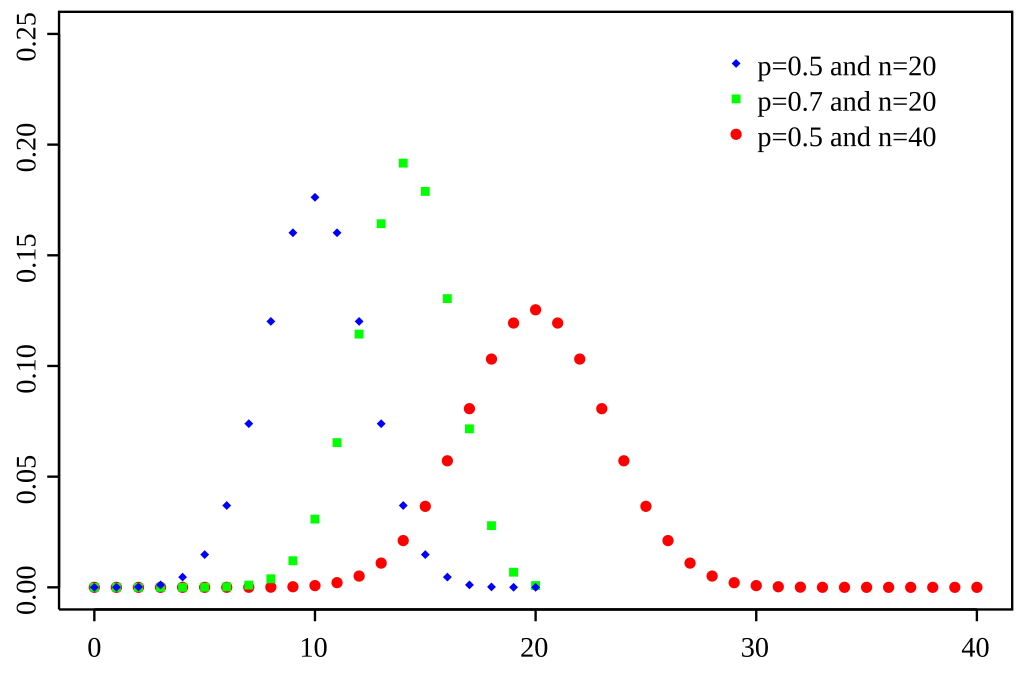
The Binomial Distribution is used to model the number of "successes" in a set of independent trials. A success could be rolling a 6 on a fair sided dice or being a carrier of a genetic condition.

The Binomial Distribution is usually characterized as X~binomial(n,p) where \(n\) independent trials are conducted and \(p\) is the probability of success for each trial. A Binomial Distribution with 1 trial \(n=1\) is also known as a Bernoulli distribution.

Some assumptions made by the Binomial Distribution:

The PMF for Binomial Distribution is \(P(X=x) = {n \choose x} p^{x}(1-p)^{n-x}\). The mean is \(np\) and the variance is \(np(1-p)\).

Normal Distribution

The Normal Distribution, also known as the Gaussian distribution, is arguably one of the most important distributions and concepts in Statistics. We typically denote the mean (which also happens to be the mode and median) as \(\mu\) and the variance as \(\sigma^2\).

The PDF of the Normal distribution is: \(P(x) = \frac{1}{\sigma\sqrt{2 \pi}} e^{-(x-\mu)^2 / 2 \sigma^2}\)

Thanks to the Central Limit Theorem, we can use the Normal distribution to approxiamate most unknown probability distributions with a large enough sample size.

Central Limit Theorem: If we draw \(n\) independent and identically distributed random variables where \(\mu\) is the true average and \(S_n\) is the sample average, then as \(n\) approaches infinity, \(\sqrt{n} (S_n - \mu)\) will converge to a Normal Distribution with mean of 0 and unknown variance, \(N(0, \sigma^2)\).

We can simplify the Central Limit Theorem to illustrate that the true sample mean \(\mu = \frac{X_1 + ... + X_n}{n}\) converges to \(N(S_n, \sigma^2/ n)\). This allows us to use properties of the Normal Distribution (for one, we can calculate the PDF and CDF) for tests of statistical signifiance (how extreme are the values we observed?) when we don't know the true distribution.

Thanks for reading our Mathematics lesson

Here are some additional reading(s) that may be helpful: